Illustrated Guide to Min Hashing

Suppose you’re an engineer at Spotify and you’re on a mission to create a feature that lets users explore new artists that are similar to the ones they already listen to. The first thing you need to do is represent the artists in such a way that they can be compared to each other. You figure that one obvious way to characterize an artist is by the people that listen to it. You decide that each artist shall be defined as a set of user IDs of people that have listened to that artist at least once. For example, the representation for Miles Davis could be,

The number of elements in the set is the number of users that have listened to Miles Davis at least once. To compute the similarity between artists, we can compare these set representations. Now, with Spotify having more than 271 million users, these sets could be very large (especially for popular artists). It would take forever to compute the similarities, especially since we have to compare every artist to each other. In this post, I’ll introduce a method that can help us speed up this process. We’re going to be converting each set into a smaller representation called a signature, such that the similarities between the sets are well preserved.

Toy Example

I think working with tiny examples to build intuition can be an excellent method for learning. In that spirit, now consider a toy example. Assume that we only have 3 artists and we have a total of 8 users in our dataset.

Jaccard similarity

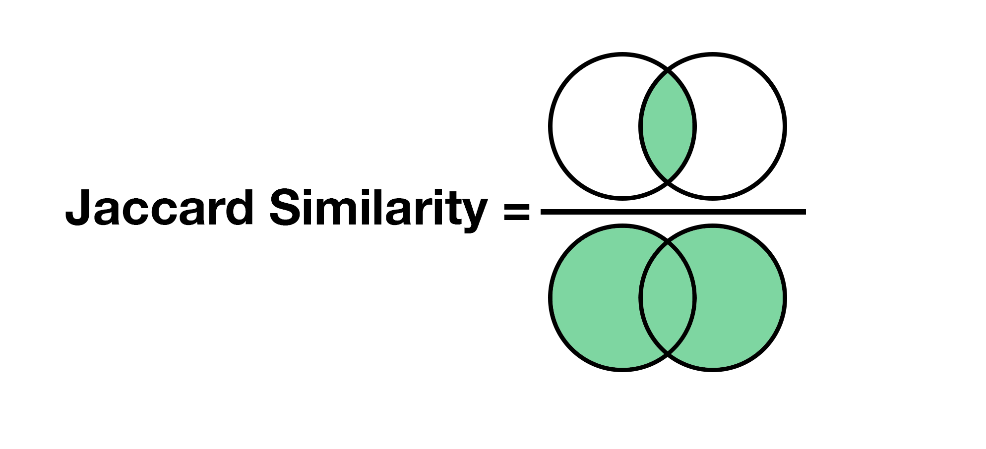
The goal is to find similar artists, so we need a way to measure similarities between a pair of artists. We will be using Jaccard similarity, it is defined as the fraction of shared elements between two sets. In our case the sets are user ids. All we have to compute is how many users each pair of artists share, divided by total number of users in both artists. For example, the Jaccard similarity between \(\text{artist}_1\) and \(\text{artist}_2\):

Similarly for the other pairs, we have:

A few key things about the Jaccard similarity:

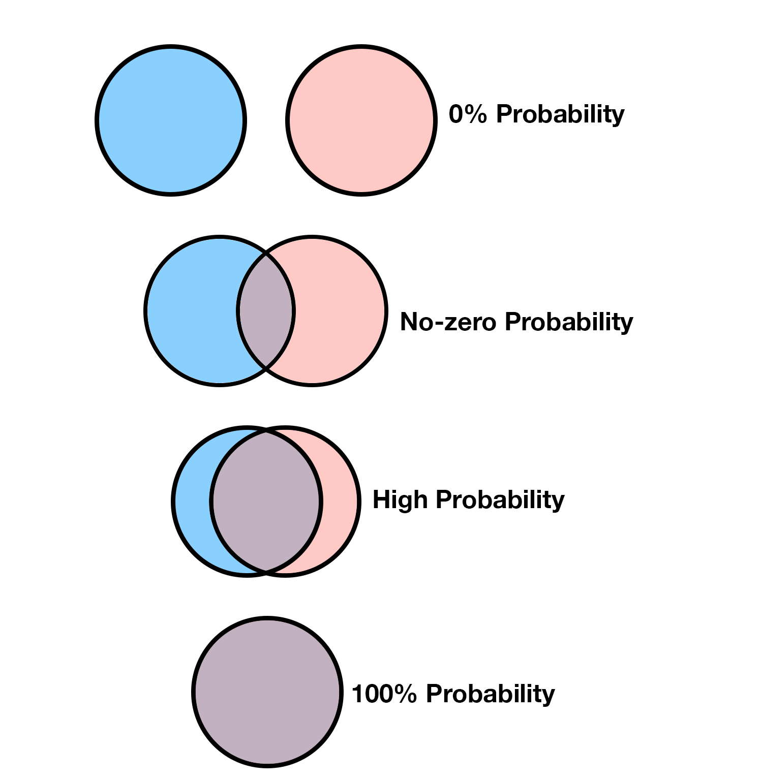
• The Jaccard similarity is 0 if the two sets share no elements, and it’s 1 if the two sets are identical. Every other case has values between 0 and 1.
• The Jaccard similarity between two sets corresponds to the probability of a randomly selected element from the union of the sets also being in the intersection.

Let’s unpack the second one, because it’s definitely the most important thing to know about the Jaccard similarity.

Intuition behind the Jaccard similarity

For some people (present company included), visual explanations are easier to grasp than algebraic ones. We’ll briefly shift our view from sets to Venn diagrams. Let’s imagine any two artists as Venn diagrams, the Jaccard similarity is the size of the intersection divided by the size of the union:

Now imagine that I’m throwing darts on the diagrams and I’m horrible at it. I’m so bad that every element on the diagrams has an equal chance of being hit. What’s the chance that I throw a dart and it lands on the intersection? It would be the number of elements in the intersection divided by the total number of elements, which is exactly what the Jaccard similarity is. This implies that the larger the similarity, the higher the probability that we land on the intersection with a random throw.

Consider another scenario. Suppose you want to know the similarity between two sets, but you can’t see the diagram, you’re blindfolded. However, if you throw a dart, you do get the information on where it landed. Can you make a good guess on the similarity of two sets by randomly throwing darts on it? Let’s say after throwing 10 darts we know that 6 of them landed in the intersection. What would you guess that the similarity of the two sets are? Let’s say after throwing 40 more darts, we know that 30 of the total 50 throws landed in the intersection. What would your guess be now? Are you more certain about your guess? Why?

Ponder about this for a little bit and keep this picture in mind throughout reading this post. This is, in essence, the basis for the MinHash algorithm.

Approximate Jaccard similarity

In the previous paragraph, we have alluded to the fact that it’s possible to approximate the Jaccard similarity between two sets. In order to see why that’s true, we need to rehash some of things we’ve said, mathematically.

Let’s take \(\text{artist}_1\) and \(\text{artist}_2\) and their union \(\text{artist}_1 \cup \text{artist}_2 = \{0, 1, 2, 4, 5, 7\}\). Some of the elements in union are also in the intersection, more specifically \(\{1, 4, 7\}\).

Let’s replace the elements with the symbols “-“ and “+”, denoting if an element appears in the intersection or not.

If every element has an equal probability of being picked, what is the probability of drawing an element that is of type “+”? It’s the number of pluses divided by number of pluses and number of minuses.

The number of “+” corresponds to the number of elements in the intersection and the number of “+” and the number of “-“ corresponds to the total number of elements or the size of the union. Therefore,

What this means is that we can approximate the Jaccard similarity between pairs of artists. Let \(X\) be a random variable such that \(X = 1\) if we draw a plus and \(X = 0\) if we draw a minus. \(X\) is a Bernoulli random variable with \(p=J(\text{artist}_{1}, \text{artist}_{2})\). In order to estimate the similarity, we can estimate \(p\). In this case, we obviously know that \(p=0.5\) since we already computed it, but let’s assume that we don’t know this.

If we repeat the random draw multiple times and keep track of how many times a “+” type came up versus a “-“, we can estimate the parameter \(p\) for \(X\) by maximum likelihood estimation (MLE):

Where \(X_{i}\) are our observations and \(n\) is the total number of draws that were made. The larger the number of draws \(n\), the better the estimation will be.

The code below will simulate the process a 30 times and empirically compute the similarity.

import numpy as np

num_trials = 30

# Union of artist_1 and artist_2
union = np.array([0, 1, 2, 4, 5, 7])

# Intersection of artist_1 and artist_2
intersection = np.array([1, 4, 7])

# Randomly pick element
draws = np.random.choice(union, num_trials)
num_intersect = np.count_nonzero(np.isin(draws, intersection))
print(num_intersect/len(draws))

If you run the above code you should get something that is close to \(0.5\). Which, as expected, corresponds to the Jaccard similarity between \(\text{artist}_1\) and \(\text{artist}_2\). Play around with the variable \(\text{num_trials}\), what happens if you set it to 1? What about 10,000?

Shuffling and Picking First \(\equiv\) Randomly Picking

Before we move on, we need to understand one more thing. Randomly selecting an element from a set is the same thing as shuffling the set and picking the first element ¹. Everything that we have said above is also true if we, instead of randomly selecting an element, shuffled the set and picked the first element.

import numpy as np

num_trials = 30

# Union of artist_1 and artist_2
union = np.array([0, 1, 2, 4, 5, 7])

# Intersection of artist_1 and artist_2
intersection = np.array([1, 4, 7])

# Shuffle and pick first element
num_intersect = 0
for i in range(num_trials):
    np.random.shuffle(union)
    if union[0] in intersection:
        num_intersect += 1
print(num_intersect/num_trials)

The code above implements the same process that I described before, but instead of randomly picking an element, it is shuffling the elements in the union and picking the first element. If you run this, you should similarly get something that is close to \(0.5\).

Data Matrix

We have shown that it’s possible to approximate Jaccard similarity for a pair of artists using randomness but our previous method had a significant issue. We still needed to have the intersection and the union of the sets to estimate the Jaccard similarity, which kind of defeats the whole purpose. We need a way to approximate the similarities without having to compute these sets. We also need to approximate the similarities for all pairs of artists, not just a given pair. In order to do that, we’re going to switch our view of the data from sets to a matrix.

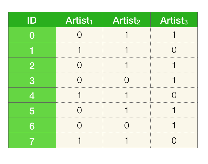
The columns represent the artists and the rows represent the user IDs. A given artist has a \(1\) in a particular row if the user with that ID has that artist in in their listening history ².

Min Hashing

Going back to our main goal, we want to reduce the size of the representation for each artist while preserving the Jaccard similarities between pairs of artists in the dataset. In more “mathy” terms, we have a data matrix \(D\) that we want to encode in some smaller matrix \(\hat{D}\) called the signature matrix, such that \(J_{pairwise}(D) \approx \hat{J}_{pairwise}(\hat{D})\)

The first algorithm I will be describing is not really practical but it’s a good way to introduce the actual algorithm called MinHash. The whole procedure can be summarized in a sentence: shuffle the rows of the data matrix and for each artist (column) store the ID of the first non-zero element. That’s it!

naive-minhashing

for k iterations
  shuffle rows
  for each column
    store the ID of first non-zero element into the signature matrix

Let’s go through one iteration of this algorithm:

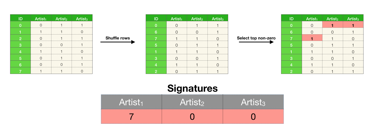
We have now reduced each artist to a single number. To compute the Jaccard similarities between the artists we compare the signatures. Let \(h\) be the function that finds and returns the index of the first non-zero element. Then we have:

And the Jaccard similarities are estimated as ³:

Why would this work?

To understand why this is a reasonable thing to do, we need to recall our previous discussion on approximating the Jaccard similarity. We were drawing elements from the union of two sets at random and checking if that element appeared in the intersection. What we’re doing here might look different, but it’s actually the same thing.

• We are shuffling the rows (thus bringing in randomness)
• By picking the first non-zero element for every artist, we’re always picking an element from the union (for any pair of artists).
• By checking if \(h(\text{artist}_{i}) = h(\text{artist}_{j})\) we are checking if the element is in the intersection
• And most importantly the probability of a randomly drawn element being in the intersection is exactly the Jaccard similarity, that is, \(P(h(\text{artist}_{i}) = h(\text{artist}_{j})) = J(\text{artist}_{i}, \text{artist}_{j})\)

Let’s go through an example together with sets \(\text{artist}_{1}\) and \(\text{artist}_{2}\). I’ve highlighted the relevant rows using the same definition for the symbols “+” and “-“ as before. We have an additional symbol called “null”, these correspond to elements that are in neither of the selected artists. The “null” type rows can be ignored since they do not contribute to the similarity (and they are skipped over in the algorithm).

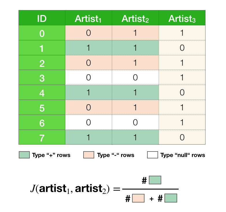
If we shuffled the rows what is the probability that the first non-“null” row is of type “+”? In other words, after shuffling the rows, if we proceeded from top to bottom while skipping over all “null” rows, what is the probability of seeing a “+” before seeing a “-“?

If we think back to our example with sets, this question should be easy to answer. All we have to realize is that, encountering a “+” before a “-“ is the exact same thing as randomly drawing a “+” in the union, which we know has a probability that is equal to the Jaccard similarity.

If the first row is of type “+” that also means that \(h(\text{artist}_{1}) = h(\text{artist}_{2})\), so the above expression is equivalent to saying:

The same argument holds for any pair of artists. The most important take away here is that if the Jaccard similarity is high between two pairs of sets, then the probability that \(h(\text{artist}_{i}) = h(\text{artist}_{j})\) is also high. Remember, throwing darts at the diagrams? It’s the same intuition here.

Now going back to our example. With a single trial we have the following estimations.

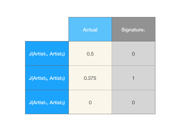
As you can see, it’s a little off. How can we make it better? It’s simple, we run more iterations and make the signatures larger. In the earlier discussions we introduced a Bernoulli random variable and we estimated it’s parameter by simulating multiple random trials. We can do the same exact thing here. Let \(Y\) be a random variable that has value 1 if \(h(\text{artist}_{i}) = h(\text{artist}_{j})\) and is 0 otherwise. \(Y\) is an instance of a Bernoulli random variable with \(p = J(\text{artist}_{i}, \text{artist}_{j})\). If we run the algorithm multiple times, thus simulating multiple but identical variables \(Y_{1}, Y_{2}, ..., Y_{k}\), we can then estimate the Jaccard similarity as:

Where \(h_{m}\) is a function that returns the first non-zero index for iteration \(m\).

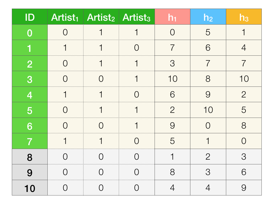
The animation below shows the process of going through 3 iterations of this algorithm:

Computing the Jaccard similarities with the larger signature matrix:

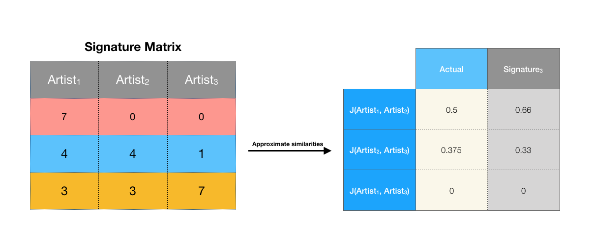
That’s much better. It’s still not exactly the same but it’s not too far off. We’ve managed to reduce the number of rows of the matrix from 8 to 3 while preserving the pairwise Jaccard similarities up to some error. To achieve a better accuracy, we could construct an even larger signature matrix, but obviously we would be trading off the size of the representation.

If you want to play around with this algorithm, here’s an implementation in Python using Numpy:

import numpy as np

def min_hashing_naive(data, num_iter):
    num_artists = data.shape[1]
    sig = np.zeros(shape=(num_iter, num_artists), dtype=int)
    for i in range(num_iter):
        np.random.shuffle(data)
        for j in range(num_artists):
            c = data[:, j]
            if np.any(c != 0):
                min_hash = np.where(c == 1)[0][0]
                sig[i, j] = min_hash
    return sig

MinHash Algorithm

Shuffling the rows of the data matrix can be infeasible if the matrix is large. In the Spotify example, we would have to shuffle 271 million rows for each iteration of the algorithm. So while the algorithm works conceptually, it is not that useful in practice.

Instead of explicitly shuffling the rows, what we can instead do is implicitly shuffle the rows by mapping each row index to some unique integer. There are special functions called hash functions that can do exactly that. They map each unique input to some unique output (usually in the same range).

Although it’s not a necessary for the range of the hash values to be the same as the indices, let’s assume for the sake of this example that it is. Then you can think of these permutations as, where the row would have landed if we actually randomly shuffled the rows. For example if we had some hash function \(h\) and applied it to row index 4:

The way you can interpret this is, the row at position 4 got moved to position 2 after shuffling.

To simulate multiple iterations of implicit shuffling, we’re going to apply multiple distinct hash functions \(h_{1}, h_{2}, ..., h_{k}\) to each row index.

Recipe for generating hash functions

Pick a prime number \(p \ge m\) where \(m\) is the number of rows in the dataset. Then each hash function \(h_{i}\) can be defined as:

Where \(a_{i}, b_{i}\) are random integers in the range \([1, p)\) and \([0, p)\), respectively. The input \(x\) to the function is the index of the row. To generate a hash function, all we have to do is pick the parameters \(a\) and \(b\).

For example, let’s define three hash functions: \(h_{1}, h_{2}, h_{3}\)

We’ll be applying these hash functions to the rows of our toy dataset. Since the number of rows \(m = 8\) is not a prime number we chose \(p = 11\). As I’ve mentioned before, the values of the hash function need not be in the same range as the indices. As long as each index is mapped to a unique value, the range of the values actually makes no difference. If this doesn’t make sense to you, let’s unpack the example we have. In this case, our hash functions will produce values in the range \([0, 10]\). We can imagine expanding our dataset with a bunch of “null” type rows so that we have \(p=11\) rows. We know that the “null” rows don’t change the probability of two artists having the same signature, therefore our estimates should be be unaffected.

Since each hash function defines an implicit shuffling order, we can iterate over the rows in that order. As an exercise, iterate the rows in the defined orders of each hash function. For each column (artist) store the index of the first-non zero element. Then to compute the Jaccard similarities, compare the stored values the same way we did before. ⁴

The MinHash algorithm is essentially doing the same thing but in a more efficient way by just making a single pass over the rows.

MinHash

Initialize all elements in the signature matrix sig to infinity
for each row r in the dataset
  Compute h_{i}(r) for all hash functions h_{1}, h_{2}, ..., h_{k}
  for each non-zero column c in the row r
    if sig(i, c) > h_{i}(r)
      update sig(i, c) = h_{i}(r)

When the algorithm terminates the signature matrix should contain all the minimum hash values for each artist and hash function pair.

The video below is an animation that simulates the algorithm over the toy dataset. Watching it should hopefully clear up any questions you have about how or why the algorithm works.

Now with this algorithm we can reduce all of the artist representations to smaller sets. If we use \(k\) hash functions we will have a signature of size \(k\) for each artist. This means that the time complexity of comparing two sets (artists) is now \(O(k)\), which is independent of the size of the original sets.

Next Steps

Using the MinHash algorithm, we can reduce the computational complexity of computing similarities between pairs of artists but there is still one more issue. In order to implement the recommendation feature we still need to compute the similarities between every pair of artists. This is quadratic in running time, if \(n\) is the number of artists, we need to make \({n \choose 2} = \frac{n(n-1)}{2} = O(n^2)\) comparisons. If \(n\) is large, even with parallelization, this will be a horribly slow computation.

We’re in luck because there’s another ingenious method called Locality-sensitive hashing (LSH) that uses the minhash signatures to find candidate pairs. This means that we’ll only have to compute the similarities for the candidates, rather than for every pair. I’ll write about LSH in the next post. Until then, .

Further reading

• Min Hashing - Lecture notes from University of Utah CS 5140 (Data Mining) by Jeff M Phillips. This is were I actually learned about Min Hashing. Answers an important question that I have not addressed in this tutorial, “So how large should we set k so that this gives us an accurate measure?”
• Finding Similar Items - Chapter 3 of the book “Mining of Massive Datasets” by Jure Leskovec, Anand Rajaraman and Jeff Ullman. Has some really good exercises that are worth checking out.

If you have any questions or you see any mistakes, please feel free to use the comment section below.