Introduction to Neural Networks
-
This post is best suited for people who are familiar with linear classifiers. I will also be assuming that the reader is familiar with gradient descent.
-
The goal of this post isn’t to be a comprehensive guide about neural networks, but rather an attempt to show an intuitive path going from linear classifiers to a simple neural network.
There are many types of neural networks, each having some advantage over others. In this post, I want to introduce the simplest form of a neural network, a Multilayer Perceptron (MLP). MLPs are a powerful method for approximating functions and it’s a relatively simple model to implement.
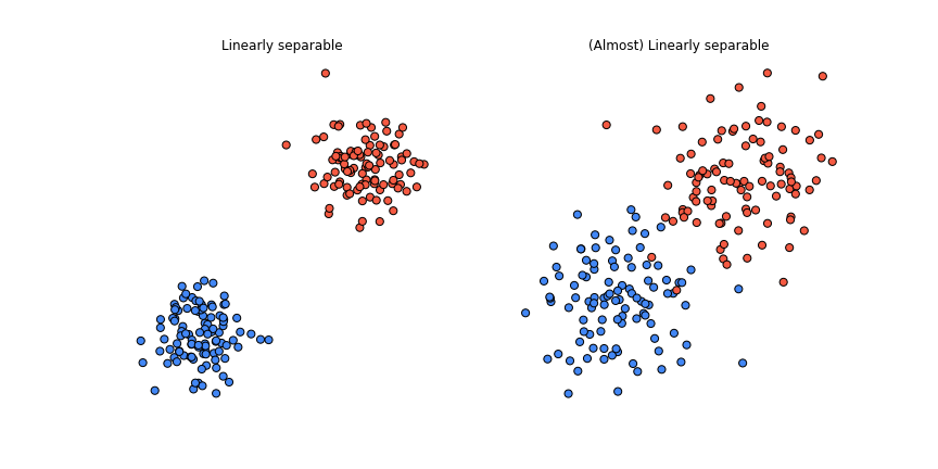
Before we delve into MLPs, let’s quickly go over linear classifiers. Given training data as pairs \((\boldsymbol{x}_i, y_i)\) where \(\boldsymbol{x}_i \in \mathbb{R}^{d}\) are datapoints (observations) and \(y_i \in \{0, 1\}\) are their corresponding class labels, the goal is to learn a vector of weights \(\boldsymbol{w} \in \mathbb{R}^{d}\) and a bias \(b \in \mathbb{R}\) such that \(\boldsymbol{w}^T\boldsymbol{x}_{i} + b \ge 0\) if \(y_{i} = 1\) and \(\boldsymbol{w}^T\boldsymbol{x}_{i} + b < 0\) otherwise (\(y_{i} = 0\)). This decision can be summarized as the following step function:
\[\text{Prediction} = \begin{cases} 1 & \boldsymbol{w}^T\boldsymbol{x} + b \ge 0 \\ 0 & \text{Otherwise}\\ \end{cases}\]In the case of Logistic Regression the decision function is characterized by the sigmoid function \(\sigma(z) = \frac{1}{1+e^{-z}}\) where \(z = \boldsymbol{w}^T\boldsymbol{x} + b\)
\[\text{Prediction} = \begin{cases} 1 & \sigma(z) \ge \theta \\ 0 & \text{Otherwise}\\ \end{cases}\]Where \(\theta\) is a threshold that is usually set to be 0.5.
If the dataset is linearly separable, this is all fine since we can always learn \(\boldsymbol{w}\) and \(b\) that separates the data perfectly. We’re in good shape even if the dataset isn’t perfectly linearly separable, i.e the data points can be separated with a line barring a few noisy observations.
But what can we do if the dataset is highly non-linear? For example, something like this:
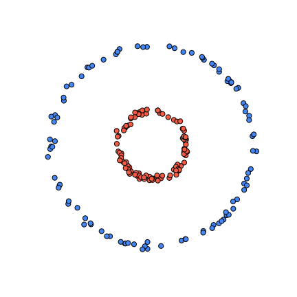
One thing we could potentially do is to come up with some non-linear transformation function \(\phi(\boldsymbol{x})\), such that applying it renders the data linearly separable. Having this transformation function would allow us to use all the tools we have for linear classification.
For example, in this case, we can see that the data points come from two concentric circles. Using this information we define the following transformation function: \(\phi(\boldsymbol{x}) = [x_1^2, x_2^2]\)
Now we can learn a vector \(\boldsymbol{w}\) and bias \(b\) such that \(\boldsymbol{w}^T\phi(\boldsymbol{x}_{i}) + b \ge 0\) if \(y_{i} = 1\) and \(\boldsymbol{w}^T\phi(\boldsymbol{x}_{i}) + b < 0\) otherwise.
![]()
This works for this particular case since we know exactly what the data generation process is, but what can we do when the underlying function is not obvious? What if we’re working in high dimensions where we can’t visualize the shape of the dataset? In general, it’s hard to come up with these transformation functions.
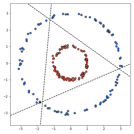
Here’s another idea, instead of learning one linear classifier, let’s try to learn three linear classifiers and then combine them to get something like this:
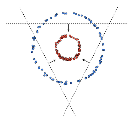
We know how to learn a single linear classifier but how can we learn three linear classifiers that can produce a result like this? The naive approach would be to try to learn them independently using different random initializations and hope that they converge to something like what we want. However, this approach is doomed from the beginning since each classifier will try to fit the whole data while ignoring what the other classifiers are doing. In other words there will be no cooperation since none of the classifiers will be “aware” of each other. This is the opposite of what we want. We want/need the classifiers to work together.
This is where MLPs come in. A simple MLP can actually do both of the aforementioned things. It can learn a non-linear transformation that makes the dataset linearly separable and it can learn multiple linear classifiers that cooperate.
The goal for the next section is to come up with a classifier that can potentially learn how to correctly classify the concentric circles dataset.
Design
Three Linear Classifiers
Let’s continue our idea of learning multiple linear classifiers. Define three classifiers \((\boldsymbol{w}_{1}, b_1), (\boldsymbol{w}_{2}, b_3)\) and \((\boldsymbol{w}_{3}, b_3)\), where \(\boldsymbol{w}_i \in \mathbb{R}^2\) and \(b_i \in \mathbb{R}\).
Because we want to learn all three jointly, it makes sense to combine them into a single object. Let’s stack all of the classifiers into a single matrix \(\boldsymbol{W}^{3 \times 2}\) and the biases into a vector \(\boldsymbol{b}^{3 \times 1}\), as such:
\[\boldsymbol{W} = \begin{bmatrix} \boldsymbol{w}^T_{1} \\ \boldsymbol{w}^T_{2} \\ \boldsymbol{w}^T_{3} \\ \end{bmatrix} = \begin{bmatrix} w_1^{(1)} & w_1^{(2)}\\ w_2^{(1)} & w_2^{(2)}\\ w_3^{(1)} & w_3^{(2)}\\ \end{bmatrix} \boldsymbol{b} = \begin{bmatrix} b_1 \\ b_2 \\ b_3 \\ \end{bmatrix}\]Now we need to get a classification decision from each one of the classifiers. We mentioned two types of decision functions in the beginning of the post, the step function and the sigmoid, which is basically a smooth step function. For technical reasons that will become clear in the next section, we’re gonna use the sigmoid function to produce decisions. For each pair \((\boldsymbol{w}_{i}, b_i)\), to get the prediction for a given data point we take \(\sigma(\boldsymbol{w}_{i}^T\boldsymbol{x} + b_i)\). This is not taking the advantage of having everything packed into a matrix. Instead of enumerating the classifiers one by one, we could do everything in one operation.
\[\sigma(\boldsymbol{Wx} + \boldsymbol{b}) = \begin{bmatrix} \sigma(\boldsymbol{w}_{1}\boldsymbol{x} + b_1) \\ \sigma(\boldsymbol{w}_{2}\boldsymbol{x} + b_2) \\ \sigma(\boldsymbol{w}{3}\boldsymbol{x} + b_3) \\ \end{bmatrix}\]Note: The \(\sigma\) function for vector valued functions is an element-wise operation.
This is great but so far we haven’t really solved anything. We just came up with a neat way to compute the output of all three classifiers given some input. We still need to connect them in order to create “cooperation”.
The Meta Classifier
Let’s define another linear classifier but this time instead of taking the data points as input, this classifier will take the outputs of the three classifiers as input and will output a final classification decision. In a way it’s a meta classifier since it classifies using outputs of other classifiers.
Let \(\boldsymbol{h}^{3 \times 1}\) be the output of the previous classifiers, i.e \(\boldsymbol{h} = \sigma(\boldsymbol{Wx} + \boldsymbol{b})\), then the prediction of the meta classifier \((\boldsymbol{w}_{m}, b_{m})\) is defined as: \(\sigma(\boldsymbol{w}_{m}^T\boldsymbol{h} + b_{m})\), where \(\boldsymbol{w}_{m} \in \mathbb{R}^3\) and \(b_{m} \in \mathbb{R}\).
And there it is, we finally have all the components. All three classifiers are connected, we have a way to produce a single prediction using all three of them and there is hope that coordination will happen because of the meta classifier.
Just to recap, the expression below is the function that corresponds to our MLP:
\[\text{MLP}(\boldsymbol{x}; \boldsymbol{w}_{m}, b_{m}, \boldsymbol{W}, \boldsymbol{b}) =\sigma(\boldsymbol{w}_{m}^T\sigma(\boldsymbol{Wx} + \boldsymbol{b}) + b_{m})\]Everything before the semicolon is the input of the function and everything after are the parameters of the function. Our goal is to learn the parameters.
Exercise: A question that you might have at this point is “why do we need to have a decision function applied to the three linear classifiers, can’t we directly plug the outputs to the meta classifier and produce a decision?”. I’m gonna leave the answer to that as an exercise. Remove all the \(\sigma\) functions, and simplify the expression. What do you get? Is it different than having a single linear classifier?
Learn
We have managed to define a simple MLP but we still need a way to learn the parameters of the function. The function is fully differentiable and this is no accident. As I said earlier, we chose to use the sigmoid function instead of the step-function as a decision function because of technical reasons. Well the technical reason is this: differentiability is nice and we like it because it allows us to use gradient based optimization algorithms like gradient descent.
Loss Function
Since the function is differentiable, we can define a loss function and then start optimizing with respect to the learnable parameters using gradient descent. Notice that the output of the MLP is a real number between 0 and 1. What we’re essentially doing is modeling the conditional distribution \(P(y | \boldsymbol{x})\) with a parametrized function \(MLP(\boldsymbol{x}; \theta)\) 1. This means that we can use the principle of maximum likelihood to estimate the parameters.
\[L(y, \hat{y}) = \frac{1}{n} \sum_{i=1}^n -y_i\log\hat{y_i} - (1-y_i)\log(1-\hat{y_i})\]Where \(\hat{y} = MLP(\boldsymbol{x}; \theta)\). The objective is to minimize \(L(y, \hat{y})\) 2 with respect to the learnable parameters \(\theta\).
Optimization
The plan is to use gradient descent to optimize \(L\). Remember that during gradient descent, we need take the gradient of the objective at every step of the algorithm (hence the name).
\[\theta \leftarrow \theta - \alpha \nabla_{\theta} L\]Where \(\alpha\) is the step size (learning rate).
Since \(L\) is a composition function, we will need to use the chain rule (from calculus). Furthermore, \(\theta\) isn’t a single variable, we will be optimizing with respect to 4 different variables \(\boldsymbol{w}_{m}, b_{m}, \boldsymbol{W}, \boldsymbol{b}\). We’re going to need to update each one at every step:
\(\boldsymbol{w}_{m} \leftarrow \boldsymbol{w}_{m} - \alpha * \frac{\partial L}{\partial \boldsymbol{w}_{m}}\)
\(b_{m} \leftarrow b_{m} - \alpha * \frac{\partial L}{\partial b_{m}}\)
\(\boldsymbol{W} \leftarrow \boldsymbol{W} - \alpha * \frac{\partial L}{\partial \boldsymbol{W}}\)
\(\boldsymbol{b} \leftarrow \boldsymbol{b} - \alpha * \frac{\partial L}{\partial \boldsymbol{b}}\)
Derivatives, Derivatives, Derivatives
Skip this section if you don’t care about all of the gory details of computing the partials. Although I do think that it’s a good idea to do this at least once by hand.
Now we will need to breakdown each of the partial derivatives using the chain rule. If we don’t give names to intermediate values, it will quickly get hairy. Let’s do that first.
\(\boldsymbol{s}_1 = \boldsymbol{Wx} + \boldsymbol{b}\)
\(\boldsymbol{h} = \sigma(\boldsymbol{s}_1)\)
\(s_2 = \boldsymbol{w}^T_{m}\boldsymbol{h} + b_{m}\)
\(\hat{y} = \sigma(s_2)\)
Before we start the tedious process of taking partial derivatives of a composed function, I want to remind you that the goal is to compute these four partial derivatives: \(\frac{\partial L}{\partial \boldsymbol{w}_{m}}, \frac{\partial L}{\partial b_{m}}, \frac{\partial L}{\partial \boldsymbol{W}}, \frac{\partial L}{\partial \boldsymbol{b}}\). If we have these values, we can use them to update the parameters at each step of gradient descent. Using the chain rule we can write down each of the partial derivatives as a product:
\(\frac{\partial L}{\partial \boldsymbol{w}_{m}} = \frac{\partial L}{\partial \hat{y}}\frac{\partial \hat{y}}{\partial s_2}\frac{\partial s_2}{\partial \boldsymbol{w}_{m}}\)
\(\frac{\partial L}{\partial b_{m}} = \frac{\partial L}{\partial \hat{y}}\frac{\partial \hat{y}}{\partial s_2}\frac{\partial s_2}{\partial b_{m}}\)
\(\frac{\partial L}{\partial \boldsymbol{W}} = \frac{\partial L}{\partial \hat{y}}\frac{\partial \hat{y}}{\partial s_2}\frac{\partial s_2}{\partial \boldsymbol{h}}\frac{\partial \boldsymbol{h}}{\partial \boldsymbol{s}_1}\frac{\partial \boldsymbol{s}_1}{\partial \boldsymbol{W}}\)
\(\frac{\partial L}{\partial \boldsymbol{b}} = \frac{\partial L}{\partial \hat{y}}\frac{\partial \hat{y}}{\partial s_2}\frac{\partial s_2}{\partial \boldsymbol{h}}\frac{\partial \boldsymbol{h}}{\partial \boldsymbol{s}_1}\frac{\partial \boldsymbol{s}_1}{\partial \boldsymbol{b}}\)
I know this looks complex but it really isn’t that complicated. All we’re doing is taking a partial derivative of the loss with respect to each of the learnable parameters. Since the loss is a composition function we have to use chain rule. That’s it.
We can see that \(\frac{\partial L}{\partial \hat{y}}\frac{\partial \hat{y}}{\partial s_2}\) is shared among all of them and that \(L, \hat{y}, s_2\) are all scalar variables therefore the derivatives are relatively easy to compute.
\(\frac{\partial L}{\partial \hat{y}} = \frac{\hat{y}-y}{\hat{y}(1-\hat{y})}\)
\(\frac{\partial \hat{y}}{\partial s_2} = \hat{y}(1-\hat{y})\) (Recall that \(\sigma^{'}(z) = (1-\sigma(z))\sigma(z)\))
Hence \(\frac{\partial L}{\partial \hat{y}}\frac{\partial \hat{y}}{\partial s_2} = \hat{y}-y\).
Continuing down the chain we get:
\(\frac{\partial s_2}{\partial \boldsymbol{w}_{m}} = \boldsymbol{h}\)
\(\frac{\partial s_2}{\partial b_{m}} = 1\)
\(\frac{\partial s_2}{\partial \boldsymbol{h}} = \boldsymbol{w}_{m}\)
Now since, \(\boldsymbol{h}\) and \(\boldsymbol{s_1}\) are both vectors, the partial \(\frac{\partial \boldsymbol{h}}{\partial \boldsymbol{s_1}}\) will be a matrix; however it will be a diagonal matrix.
\[\frac{\partial \boldsymbol{h}}{\partial \boldsymbol{s_1}} = \text{diag}((\boldsymbol{1} - \boldsymbol{h}) \odot \boldsymbol{h})\]This can be replaced by an element-wise multiplication in the chain as: \(\odot (\boldsymbol{1} - \boldsymbol{h}) \odot \boldsymbol{h}\)
The partial derivative \(\frac{\partial \boldsymbol{s_1}}{\partial \boldsymbol{W}}\) is the most complicated to compute. \(\boldsymbol{s_1}\) is a vector and \(\boldsymbol{W}\) is a matrix, therefore the result of the partial derivative will be a 3 dimensional tensor! Fortunately, we will be able to reduce it to something more simple.
Instead of computing the partial derivative with respect to entire weight matrix, let’s instead take derivatives with respect to each of the classifiers \(\boldsymbol{w_1}, \boldsymbol{w_2},\) and \(\boldsymbol{w_3}\) (these correspond to the rows of \(\boldsymbol{W}\)). Each of these derivatives will be a matrix instead of a tensor.
\(\frac{\partial \boldsymbol{s_1}}{\partial \boldsymbol{w_1}} = \begin{bmatrix}
x_1 && x_2\\
0 && 0 \\
0 && 0 \\
\end{bmatrix}\)
\(\frac{\partial \boldsymbol{s_1}}{\partial \boldsymbol{w_2}} = \begin{bmatrix}
0 && 0\\
x_1 && x_2 \\
0 && 0 \\
\end{bmatrix}\)
\(\frac{\partial \boldsymbol{s_1}}{\partial \boldsymbol{w_3}} = \begin{bmatrix}
0 && 0\\
0 && 0 \\
x_1 && x_2 \\
\end{bmatrix}\)
We know that we’re gonna be using these values in a multiplication. We can use this fact to simplify the expression for the derivative. Let \(\frac{\partial L}{\partial \hat{y}}\frac{\partial \hat{y}}{\partial s_2}\frac{\partial s_2}{\partial \boldsymbol{h}}\frac{\partial \boldsymbol{h}}{\partial \boldsymbol{s}_1} = \boldsymbol{\delta}\), then we’ll have
\(\boldsymbol{\delta} \frac{\partial \boldsymbol{s_1}}{\partial \boldsymbol{w_1}} = [\delta_1x_1, \delta_1x_2]\)
\(\boldsymbol{\delta} \frac{\partial \boldsymbol{s_1}}{\partial \boldsymbol{w_2}} = [\delta_2x_1, \delta_2x_2]\)
\(\boldsymbol{\delta} \frac{\partial \boldsymbol{s_1}}{\partial \boldsymbol{w_3}} = [\delta_3x_1, \delta_3x_2]\)
Which implies that \(\boldsymbol{\delta}\frac{\partial \boldsymbol{s_1}}{\partial \boldsymbol{W}} = \begin{bmatrix} \delta_1x_1 && \delta_1x_2\\ \delta_2x_1 && \delta_2x_2 \\ \delta_3x_1 && \delta_3x_2 \\ \end{bmatrix}\)
We can rewrite this compactly as an outer product between \(\boldsymbol{\delta}\) and \(\boldsymbol{x}\).
\[\frac{\partial L}{\partial \hat{y}}\frac{\partial \hat{y}}{\partial s_2}\frac{\partial s_2}{\partial \boldsymbol{h}}\frac{\partial \boldsymbol{h}}{\partial \boldsymbol{s}_1}\frac{\partial \boldsymbol{s_1}}{\partial \boldsymbol{W}} = \boldsymbol{\delta} \otimes \boldsymbol{x}\]And finally,
\[\frac{\partial \boldsymbol{s_1}}{\partial \boldsymbol{b}} = \text{diag}(\boldsymbol{1}) = \boldsymbol{I}\]Putting everything together:
\(\frac{\partial L}{\partial \boldsymbol{w}_{m}} = (\hat{y} - y)\boldsymbol{h}\)
\(\frac{\partial L}{\partial b_{m}} = \hat{y} - y\)
\(\frac{\partial L}{\partial \boldsymbol{W}} = ((\hat{y} - y)\boldsymbol{w}_{m}\odot (\boldsymbol{1} - \boldsymbol{h}) \odot \boldsymbol{h}) \otimes \boldsymbol{x}\)
\(\frac{\partial L}{\partial \boldsymbol{b}} = ((\hat{y} - y)\boldsymbol{w}_{m}\odot (\boldsymbol{1} - \boldsymbol{h}) \odot \boldsymbol{h})^T\)
You may have noticed that all of this is for a single datapoint \(\boldsymbol{x}\), we wouldn’t do this in practice. It is much more preferable to have everything computed for a batch (or mini-batch) of inputs \(\boldsymbol{X}\), this allows us to update the parameters much more efficiently. I highly recommend you redo all of the computations of the partial derivatives in matrix form.
I’ve purposefully skipped over a lot of the details. I want this block of the post to serve as a reference for your own solutions rather than a complete step-by-step guide. Here are some useful notes that can come in handy if you want to do everything from scratch:
- Vector, Matrix, and Tensor Derivatives - Erik Learned-Miller
- Computing Neural Network Gradients - Kevin Clark
Results
Phew! Now that’s over with. Let’s see what the results are after running gradient descent (1000 iterations with a learning rate of 0.01). Do you remember how we started? We said that if only we had a transformation function that could make the dataset linearly separable, then learning would be easy. Well \(\phi(\boldsymbol{x}) = \sigma(\boldsymbol{Wx} + \boldsymbol{b})\) will actually be that transformation that makes the dataset linearly separable. This is what the data looks like after applying that learned function:
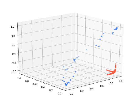
As you can see the data is completely linearly separable. In essence, this is what most of learning is when it comes to neural networks. Every neural network classifier that has classification as a primary task is trying to learn some kind of a transformation on the data so that the data becomes linearly separable. This is a big reason why neural networks became so popular. In the past, people (usually domain experts) spent tremendous efforts in engineering features to make learning easy. Now a lot of that is handled by (deep) neural networks 3.
We were also trying to learn multiple linear classifiers. And voilà, these are the three linear classifiers \((\boldsymbol{w}_{1}, b_1), (\boldsymbol{w}_{2}, b_3)\) and \((\boldsymbol{w}_{3}, b_3)\) that are learned:
Finally this is what the learned decision boundary looks like in the original space. The colors indicate the predictions of the classifier.
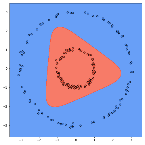
This is awesome, isn’t it? But wait, hold on. While this classifier gets 100% accuracy, it does not represent the true function… with three classifiers, the shape we are learning is a triangle-ish shape. That’s because it’s the only possible shape that captures all the data with three lines. But we know that the actual function is a circle. With four classifiers we can get rectangle-ish shapes, with five a pentagon-ish and so on. Intuitively, if we add more classifiers, we should get closer to an actual circle. Here’s a progression of the decision boundary going from 5 to 50 with increments of 5:
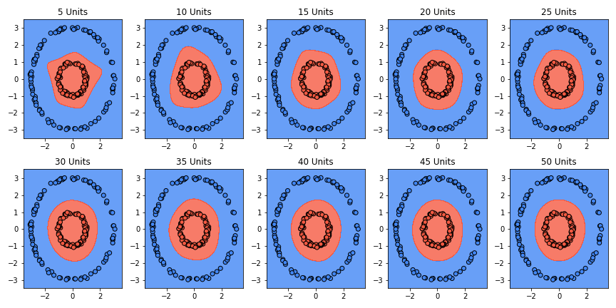
This looks much better. Yet this isn’t really the true function either. Everything in the middle is classified as red, but there will never be any points there. The true function generates points on the boundary of the circle, never inside the circle. Furthermore, the only reason we were able to make this correction was because we’re working in 2 dimensions and we know exactly what the true function is. What do we do if we have a dataset in high dimensions coming from an unknown function? Would we be able to trust the learned classifier even if we get 100% accuracy?
Jargon
For the entirety of the post, I have purposefully avoided mentioning neural network lingo that you usually see in the literature. I think some of the terms themselves can bring a lot of confusion to people when they first get introduced to neural networks. However, since the field is set on using these terms, it’s necessary to know them. Let’s go back and put names on some of the things we’ve talked about.
Activation Functions
We talked about decision functions. We mentioned the step function and the sigmoid function. The justification for having them was straight-forward since we were talking in the context of classifiers and we had to have a function that produces a prediction. In the context of neural networks we don’t really care for predictions if it isn’t the last classifier (the meta-classifier). Every intermediate function can have any form, as long as it’s differentiable.
Because of this, we aren’t constrained to using functions that produce predictions like sigmoid or the step function. Here are a few others we could have used: Tanh, ReLu, LeakyReLu, SoftPlus etc. People refer to these functions as activation functions. The most popular choice in practice is the ReLu activation defined as \(\text{ReLu}(z)=\max(0, z)\). Activation functions are almost always non-linear. The non-linearity is the reason why neural networks are able to learn non-linear functions. When the input is a vector or a matrix, the activation function is applied element-wise.
Unit (Neuron)
As we mentioned above, we don’t really need to predict in the intermediate operations. Therefore, we probably shouldn’t be calling these functions classifiers. People usually call these functions neurons or units. I prefer to call them units since calling to them neurons is drawing a parallel to biological neurons which are not similar at all. A unit takes the following form:
\[g(\boldsymbol{w}^T\boldsymbol{x} + b) = y\]Where \(g\) is some (usually non-linear) activation function.
Layer
A layer in the context of an MLP is a linear transformation followed by an activation function. A bunch of neurons together on the same level make a layer. What a level means will be more clear when we see the graphical representation of neural networks.
In this post, we defined a 2 layer MLP.
- Layer 1: Linear transformation \(\boldsymbol{Wx} + \boldsymbol{b} = \boldsymbol{s}_1 \rightarrow\) activation \(\rightarrow \sigma(\boldsymbol{s}_1) = \boldsymbol{h}\)
- Layer 2: Linear transformation \(\boldsymbol{w}_{m}^T\boldsymbol{h} + b_{m} = \boldsymbol{s}_2 \rightarrow\) activation \(\sigma(\boldsymbol{s}_2) \rightarrow \hat{y}\)
People refer to the layers before the last layer as hidden layers. In this case, we only had one hidden layer (Layer 1).
More layers: In practice, we usually have many such layers with each connected to each other, i.e the output of one becomes the input for to next one. Chaining layers like this is actually the same as function composition. If we define each layer as a function \(f_i(x) = g(\boldsymbol{W}_i\boldsymbol{x} + \boldsymbol{b}_i)\) where \(g\) is some activation function, then an n-layer MLP can be written as the function composition \(MLP(x) = f_n(f_{n-1}(...(f_1(x)))\). The depth of a network corresponds to \(n\). A network with depth \(n > 2\), is called deep (this is where the term deep learning comes from). The width of a network corresponds to the number of units in each of the layer.
Graph
You may have been confused about the fact that MLP is called a neural network. So far we haven’t seen the “network” part. The MLP that we defined can equivalently be represented by a directed acyclic graph (DAG).
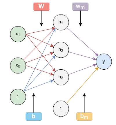
These kinds of graphs are called computational graphs and they are just another way to describe a neural network model. It provides a good way to break down a complex computation into its’ primitive parts.
All of the edges correspond to the weights (parameters) of the model. The nodes represent computation. For example, \(h_1\) represents the following computation:
\[h_{1} = \sigma(\boldsymbol{w}_{1}^T\boldsymbol{x} + b_{1})\]Edges coming out of the node that have a 1 on it are the biases.
To make sense of the rest of the edges, let’s highlight a path of a single unit \((\boldsymbol{w_1}, b_{1})\) to the output:
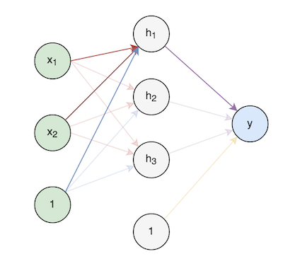
This representation is useful for computing gradients. If we wanted to take the derivative of the loss with respect to the first unit, the highlighted path tells us that we have to start from the last output and work our way backwards until we reach the desired variables.
In this post we calculated all of the gradients by hand but in practice this is done through the algorithm known as backpropagation. It works by repeatedly applying the chain rule to compute all the gradients.
Forward pass: Running through the graph and computing all the values is called the forward pass. It’s called forward pass because we’re traveling from the first layer to the last.
Backward pass: Computing the derivatives of all the parameters with respect to the outputs is called a backward pass. Similar to forward pass, the backward pass is called backward because we’re traversing starting from the last layer and working our way back.
Final Words
I hope this post has provided some insight to you on how neural networks work. It is by no means comprehensive, I have skipped over a lot of details. If you want to continue learning about neural networks, I would recommend the Deep Learning book by Ian Goodfellow and Yoshua Bengio and Aaron Courville as a good place to start. Here are a few other good resources:
- Neural Network Playground - One of the best ways to learn something is to play around with it. The NN playground lets you easily build and train models on various synthetic datasets. Great tool for building intuition.
- CS231n: Convolutional Neural Networks for Visual Recognition - Contains excellent notes from Andrej Karpathy, highly recommended.
- CSC 321: Intro to Neural Networks and Machine Learning - This has more than just neural networks. The lecture slides and notes are really good and it builds up from linear classifiers.
- 3Blue1Brown: Neural Networks - One of my all time favorite educational channels. Has some amazing, visual heavy explanations on the concepts behind neural networks.
Code
What’s a tutorial without code, am I right? Here is a link to the Jupyter notebook that contains all the code for this post.
-
To simplify the notation I’m referring to all of the parameters \(\boldsymbol{w}_{m}, b_{m}, \boldsymbol{W}, \boldsymbol{b}\) with just \(\theta\). ↩
-
What we have written here is the negative log-likelihood. Some people refer to this loss function as binary cross-entropy loss. These are equivalent loss functions, the only difference is the method/assumptions that one uses to arrive at each. ↩
-
There are downsides to this, I’ll write a post about this in the future (hopefully). ↩