Locality Sensitive Hashing for MinHash
In the previous post we covered a method that approximates the Jaccard similarity by constructing a signature of the original representation. This allowed us to significantly speed up the process of computing similarities between sets. But remember that the goal is to find all similar items to any given item. This requires to compute the similarities between all pairs of items in the dataset. If we go back to our example, Spotify has about 1.2 million artists on their platform. Which means that to find all similar artists we need to make 1.4 trillion comparisons… ahm … how about no. We’re going to do something different. We’re instead going to use Locality Sensitive Hashing (LSH) to identify candidate pairs and only compute the similarities on those. This will substantially reduce the computational time.
LSH is a neat method to find similar items without computing similarities between every possible pair. It works by having items that have high similarity be hashed to the same bucket with high probability. This allows us to only measure similarities between items that land in the same bucket rather than comparing every possible pair of items. If two items are hashed to the same bucket, we consider them as candidate pairs and proceed with computing their similarity.
Banding Technique
LSH is a broad term that refers to the collection of hashing methods that preserve similarities. In this post we’re going to be discussing one particular such method that efficiently computes candidate pairs for items that are in the form of minhash signatures. It is a pretty easy procedure both algorithmically and conceptually. It uses the intuition that if two items have identical signature parts in some random positions then they’re probably similar. This is the idea we’re going to turn to in order to identify candidate pairs.
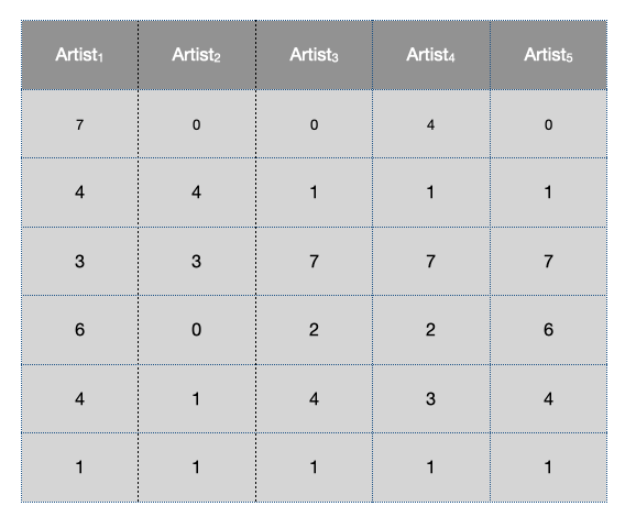
In order to proceed we first need a signature matrix, if you don’t recall how a signature matrix is computed you can refer to my previous post on min hashing. Let’s assume that a signature matrix is provided to us:
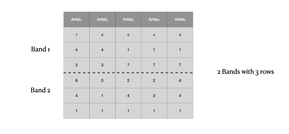
We begin by dividing the signature matrix into \(b\) bands with \(r\) rows. This means that we are slicing each item’s signature into contiguous but distinct chunks.
For each band, we take all of the chunks and hash them individually using some hashing function 1 and we store them into a hash bucket. An important thing to note is that we use a separate hash bucket for each of the bands, this makes sure that we only compare chunks of signatures within the same bands rather than across bands. The idea is that if two items land in the same bucket for any of the bands then we consider them as candidates. Using a hashing function rather than directly comparing the items is what allows us to avoid the quadratic amount of comparisons.
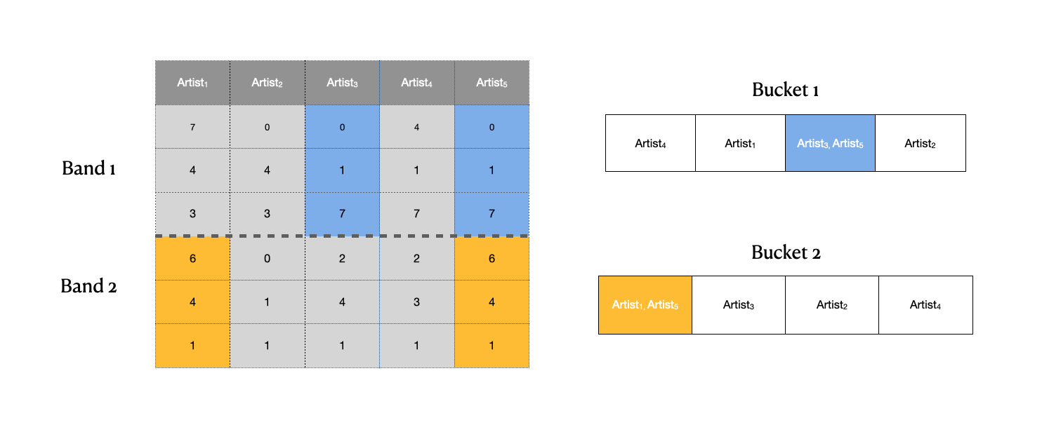
In this case it looks like we have the following candidate pairs: \((\text{artist}_{3}, \text{artist}_{5})\) and \((\text{artist}_{1}, \text{artist}_{5})\).
Note: Although the picture depicts a hash table with only four buckets in reality the number of buckets is usually much larger than the number of items.
Here’s a really simple implementation of an LSH for Jaccard similarities:
from collections import defaultdict
import numpy as np

def minhash_lsh(sig_matrix, num_bands):
    num_rows = sig_matrix.shape[1]
    bands = np.split(sig_matrix, num_bands)
    bands_buckets = []
    for band in bands:
        items_buckets = defaultdict(list)
        items = np.hsplit(band, num_rows)
        for i, item in enumerate(items):
            item = tuple(item.flatten().astype(int))
            items_buckets[item].append(i)
        bands_buckets.append(items_buckets)

    return bands_buckets
Now you may have noticed that \(b\) and \(r\) are parameters that we completely arbitrarily picked. To understand the significance of them we have to go back a little bit. Recall that the probability of two items having the same min hash value in any of the rows of the signature matrix is equal to the Jaccard similarity of those two items. We can use this fact to compute the probability of these two items being candidate pairs. Let \(s\) be the Jaccard similarity, then:
- If each band has \(r\) rows, the probability that the signatures agree on the entire band is: \(s^r\)
- The inverse of this, the probability that they do not agree is \(1 - s^r\)
- The probability that the signatures disagree in all of the bands \((1 - s^r)^b\)
- Therefore, the probability that the two items signatures agree in at least one band is \(1 - (1 - s^r)^b\)
We have just derived the probability of two items being a candidate pair as a function of \(s\) with parameters \(r\) and \(b\): \(f_{b, r}(s) = 1 - (1 - s^r)^b\). If you plot this function using any \(b\) and \(r\) it will look like an S curve.
For example, let’s plot the function with parameters \(b=2\) and \(r=3\).
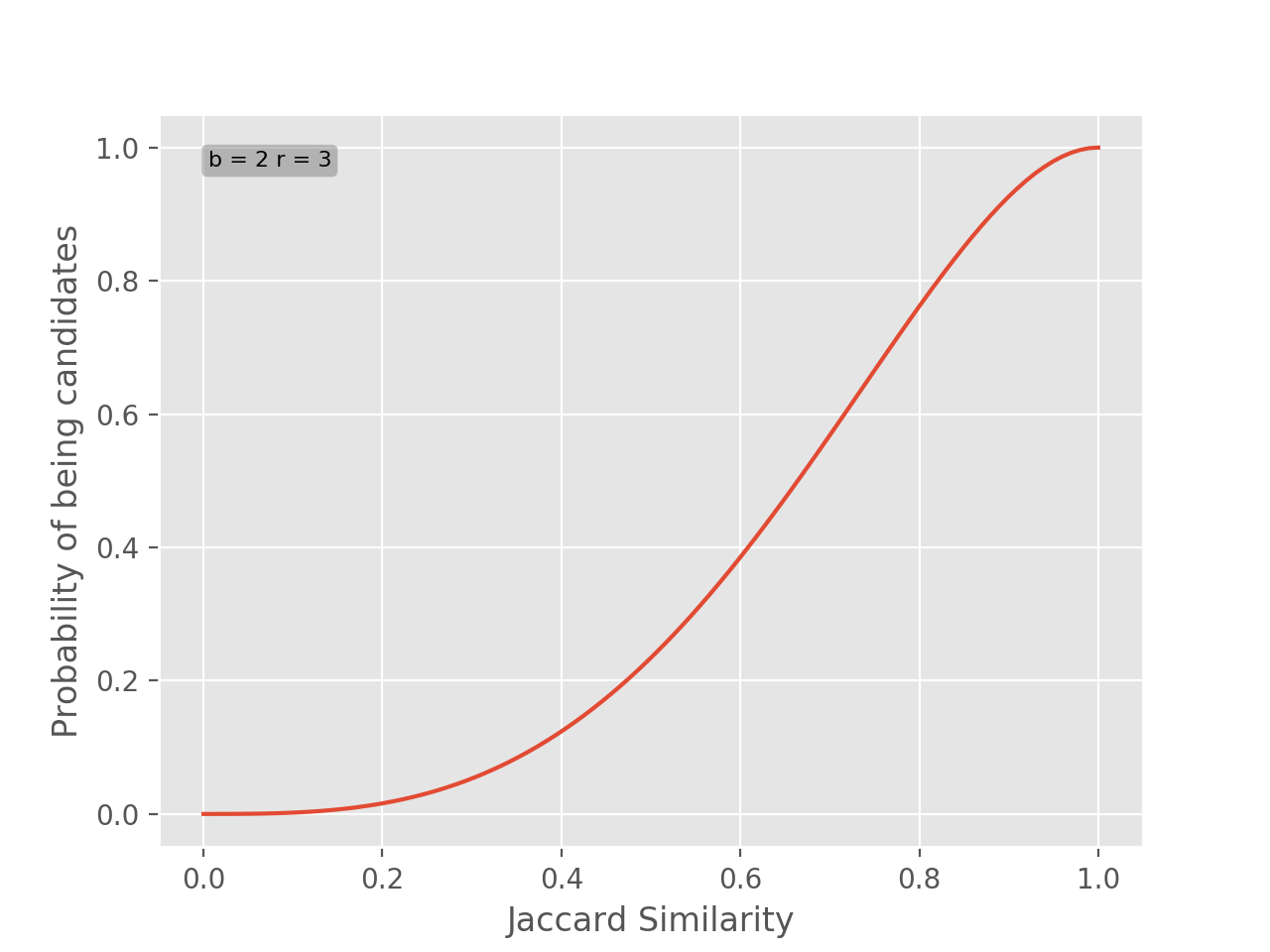
As we can see the plot is shifted to right side, this means that in order for two items be candidates their similarities have to be high. For example, if two items have similarity of \(0.5\) they only have \(0.23\) probability of being candidates. If you go back and look at the signature matrix this should make perfect sense, we selected parameters that produce large bands relative to the signature matrix. If we wanted to make it more probably for candidates to appear, we can increase \(b\).
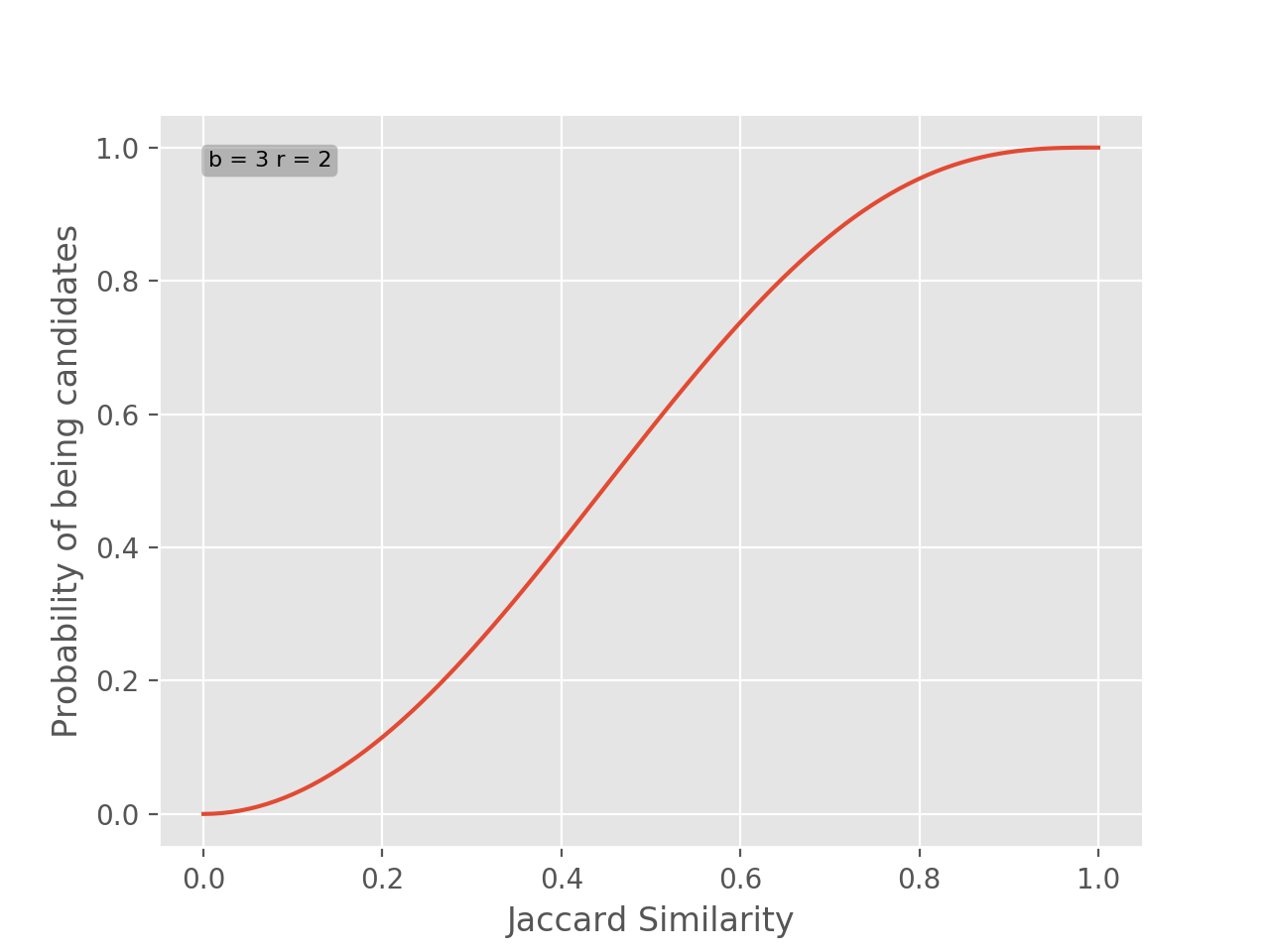
Notice how the plot has shifted to the left. With these parameters if two candidates have similarity \(0.5\) we have \(0.57\) probability of them being candidates.
In the beginning of the post I mentioned that we would only cover a single instance of an LSH method. The method we described can work really great for approximating nearest neighbours when your data points are sets but what if our data points are vectors in some high dimensional space? Luckily, there are methods that work on other types of data. Check out Chapter 3.6 of Mining Massive Datasets if you want to know more about what LSH is formally and what other techniques are there.
-
We can use the built-in hashing function of whatever programming language we’re using. ↩